Machine Learning: Maths and Definitions

Introduction

The following provides definitions that are useful in Machine Learning.

Definitions

Real Number (Mathematics)

A real number is a value that can represent a distance along a line.

Rational Number (Mathematics)

A rational number is a value that can be written as a ratio. That means it can be written as a fraction, in which both the numerator (the number on top) and the denominator (the number on the bottom) are whole numbers (also known as an integer), and the denominator is not equal to zero.

Complex Number (Mathematics)

A complex number is a combination of a Real Number and an Imaginary Number. The standard format for complex numbers is a + bi, with the real number first and the imaginary number last. Because either part could be 0, technically any real number or imaginary number can be considered a complex number. Complex does not mean complicated; it means that the two types of numbers combine to form a complex, like a housing complex — a group of buildings joined together.

Set (Mathematics)

A set is a collection of distinct objects that are considered to be an object in its own right. For example, the real numbers 2, 4, and 6 are distinct objects when considered separately, but when they are considered collectively they form a single set of size three, written {2,4,6}.

A set of real numbers is represented by the ℝ symbol, a set of rational numbers is represented by the ℚ symbol, and a set of complex numbers is represented by the ℂ symbol.

Element or Member (Mathematics)

An element, or member, of a set is any one of the distinct objects that make up that set. In the above example, 2,4 and 6 are the individual elements, or members.

Closure (Mathematics)

A set has closure under an operation if performance of that operation on members of the set always produces a member of the same set.

Associativity (Mathematics)

As set has associativity if it does not matter how we order/group the members.

Identity (Mathematics)

An identity element, or neutral element, is a special type of element of a set with respect to a binary operation on that set, which leaves other elements unchanged when combined with them. In other words, it is an equality relation A = B, such that A and B contain some variables and A and B produce the same value as each other regardless of what values (usually numbers) are substituted for the variables. In other words, A = B is an identity if A and B define the same functions.

Invertibility (Mathematics)

The idea of an inverse element generalizes concepts of a negation (sign reversal) in relation to addition, and a reciprocal in relation to multiplication.

Group (Mathematics)

A group is a structure consisting of a set of elements equipped with an operation that combines any two elements to form a third element and that satisfies four conditions called the group axioms, namely closure, associativity, identity and invertibility. One of the most familiar examples of a group is the set of integers together with the addition operation.

Commutative Group (Mathematics)

A commutative group, also known as an abelian group, is a group in which the result of applying the group operation to two group elements does not depend on the order in which they are written.

Distributive Property (Mathematics)

The distributive property is an algebra property which is used to multiply a single term and two or more terms inside a set of parentheses. The distributive property tells us that we can remove the parentheses if the term that the polynomial is being multiplied by is distributed to, or multiplied with, each term inside the parentheses. So, if we start with 6(2 + 4x) we can apply the distributive property giving us 6 * 2 + 6 * 4x. The parentheses are removed and each term from inside is multiplied by the six, which we can now simplify to 12 + 24x. It is really a law about replacement.

Field (Mathematics)

Loosely, a field is a set of elements where you can add, subtract, multiply and divide, and everything is commutative (which means things can be moved around without changing the result). Subtraction is really the same thing as adding negative numbers and division is the same thing as multiplying by fractions. So technically, a field is a set of elements, along with two operations defined on that set: an addition operation written as a + b, and a multiplication operation written as a ⋅ b. A field is commutative group under addition and multiplication, if you omit zero, and they are a distributive property.

The best known fields are the field of rational numbers, the field of real numbers and the field of complex numbers.

Scalar (Mathematics)

As outlined in vector space below, a scalar is an element of a field which is used to define a vector space. Scalars are quantities that are fully described by a magnitude alone, they have no direction (they are one dimensional). Sometimes scalar is used informally to mean a vector, matrix, tensor, or other usually “compound” value that is actually reduced to a single component. For example, the product of a 1×n matrix and an n×1 matrix, which is formally a 1×1 matrix, is often said informally to be a scalar. A scalar is also a rank-0 tensor.

Vector (Mathematics)

A quantity described by multiple scalars, such as having both direction and magnitude, is called a vector. In a plane, the direction and magnitude are described as the coordinates and it is assumed that the tail of the vector is at the origin and that the head of the vector is at the given coordinates. You can think of a vector of dimension n as an ordered collection of n elements, called components. A vector is also a rank-1 tensor.

Matrix (Mathematics)

A matrix is a rectangular array of numbers, symbols, or expressions, arranged in rows and columns. A matrix is also a rank-2 tensor.

Tensor (Mathematics)

Tensors are geometric objects that describe linear relations between geometric vectors, scalars, and other tensors. Elementary examples of such relations include the dot product, the cross product, and linear maps. The tensor is a more generalized form of scalar and vector. Or, the scalar, vector are the special cases of tensor. If a tensor has only magnitude and no direction (rank-0 tensor), then it is called scalar. If a tensor has magnitude and one direction (rank-1 tensor), then it is called vector.

Often, and erroneously, used interchangeably with the matrix, which is specifically a 2-dimensional tensor, tensors are generalizations of matrices to n-dimensional space. Mathematically speaking, tensors are more than simply a data container, however. Aside from holding numeric data, tensors also include descriptions of the valid linear transformations between tensors. Examples of such transformations, or relations, include the cross product and the dot product. From a computer science perspective, it can be helpful to think of tensors as being objects in an object-oriented sense, as opposed to simply being a data structure.

Tensor (Machine Learning)

From a Machine Learning perspective, a tensor is a generalization of vectors and matrices and is easily understood as a multidimensional array. In the general case, it is an array of numbers (a container) arranged on a regular grid with a variable number of axes is known as a tensor.

Tensor (TensorFlow)

TensorFlow, is a framework to define and run computations involving tensors, which are represented as n-dimensional arrays of base datatypes. In TensorFlow the main object you manipulate and pass around is a Tensor, which is an object that represents a partially defined computation that will eventually produce a value. TensorFlow programs are graphs of Tensor objects detailing how each tensor is computed based on the other available tensors and then by running parts of this graph to achieve the desired results. Each element in the Tensor has the same data type, and the data type is always known. The shape (that is, the number of dimensions it has and the size of each dimension) might be only partially known. Most operations produce tensors of fully-known shapes if the shapes of their inputs are also fully known, but in some cases it’s only possible to find the shape of a tensor at graph execution time. The rank of a Tensor object is its number of dimensions. Synonyms for rank include order or degree or n-dimension.

Vector Space (Mathematics)

A vector space, which is also called a linear space, is a collection of vectors; vectors are elements in a vector space. You can add any two vectors to get a third vector, and if you multiply the coordinates by a number (the scalar) you can scale the vector. So, a vector space is a collection of vectors which may be added together and multiplied (scaled) by numbers called scalars (this is where scalar gets its name, it scales). In a two dimensional vector space the vector’s coordinates are described using 2 scalars and in a three dimensional vector space the coordinates are described using 3 scalars. A n-dimensional space is called a n-space.

In vector spaces you can add any two vectors, vector addition is commutative, there is a zero vector, you can add the zero vector to any vector and the vector remains unchanged (making the zero vector an identity element), for every vector there is a vector pointing in the opposite direction (which when added together gives you the zero vector), and vector addition is associative (it does not matter how we order/group the vectors).

Cartesian Coordinate (Mathematics)

A cartesian coordinate graph is made up of two axes (“axes” is just the plural of “axis”). The horizontal axis is called the x-axis, or x-coordinate, and the vertical one is the y-axis, or y-coordinate. When describing it, the x-coordinate always comes first, followed by the y-coordinate.

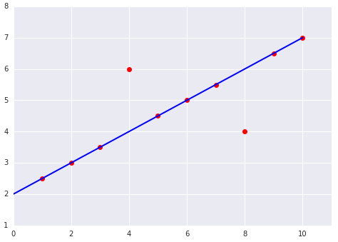
Linear Regression (Mathematics)

In statistics, linear regression is a linear approach to modeling the relationship between a scalar response and one or more explanatory variables. The term linear means that it can be graphically represented along a straight, or nearly straight, line.

A scalar response, also known as dependent variables, represents the output or outcome whose variation is being studied.

Explanatory variables, also known as independent variables, represent the inputs or causes that are potential reasons for variation. If you have one explanatory variable it is called simple linear regression and if you have more than one explanatory variable then the process is called multiple linear regression.

So, linear regression is simply the process of modeling the relationship between inputs and outputs. A linear regression tries to estimate a linear relationship that best fits a given set of data.

Linear regression is distinct from multivariate linear regression, where multiple correlated dependent variables are predicted, rather than a single scalar variable.

Bias (Mathematics)

An intercept or offset from an origin.

Derivative (Mathematics)

Derivative is a way to show rate of change: that is, the amount by which a function is changing at one given point.

Partial Derivative (Mathematics)

A partial derivative of a function of several variables is its derivative with respect to one of those variables, with the others held constant (as opposed to the total derivative, in which all variables are allowed to vary).

Machine Learning (Machine Learning)

Supervised Machine Learning (ML) learns how to combine labeled input data to produce useful predictions on never-before-seen data. In unsupervised ML, all data is unlabeled and the algorithms learn to inherent structure from the input data.

Label (Machine Learning)

A label is the thing we’re predicting, the y variable in simple linear regression. The label could be the future price of wheat, the kind of animal shown in a picture, the meaning of an audio clip, or just about anything.

Feature (Machine Learning)

A feature is an input variable, the x variable in simple linear regression. A simple ML project might use a single feature, while a more sophisticated machine learning project could use millions of features.

Examples (Machine Learning)

An example is a particular instance of data, x (we put x in boldface to indicate that it is a vector.) We break examples into two categories:

• Labeled examples.
• Unlabeled examples

A labeled example includes both feature(s) and the label. That is:

labeled examples: {features, label}: (x, y)

You use labeled examples to train the model. In our spam detector example, the labeled examples would be individual emails that users have explicitly marked as “spam” or “not spam.”

An unlabeled example contains features but not the label. That is:

unlabeled examples: {features, ?}: (x, ?)

Once we’ve trained our model with labeled examples, we use that model to predict the label on unlabeled examples.

Training (Machine Learning)

Training means creating or learning the model. In supervised learning you show the model labeled examples and enable the model to gradually learn the relationships between features and label. The process of training a ML model involves providing a ML algorithm (the learning algorithm) with training data to learn from. The learning algorithm finds patterns in the training data that map the input data attributes to the target (the answer that you want to predict), and it outputs an ML model that captures these patterns.

So, supervised training simply means learning (determining) good values for all the weights and the bias from labeled examples.  The goal of training a model is to find a set of weights and biases that have low loss, on average, across all examples.

Inference (Machine Learning)

Inference means applying the trained model to unlabeled examples, also known as unsupervised training. That is, you use the trained model to make useful predictions (y'). For example, during inference, you can predict medianHouseValue for new unlabeled examples.  To infer means to predict.

Model (Machine Learning)

The term ML model refers to the model artifact that is created by the training process, it defines the relationship between features and label. You can use the ML model to get predictions on new data for which you do not know the target. For example, let’s say that you want to train a ML model to predict if an email is spam or not spam. You would provide training data that contains emails for which you know the target (that is, a label that tells whether an email is spam or not spam). The ML would train an ML model by using this data, resulting in a model that attempts to predict whether new email will be spam or not spam.

Regression vs Classification (Machine Learning)

A regression model predicts continuous values. For example, regression models make predictions that answer questions like the following:

• What is the value of a house in California?
• What is the probability that a user will click on this ad?

A classification model predicts discrete values. For example, classification models make predictions that answer questions like the following:

• Is a given email message spam or not spam?
• Is this an image of a dog, a cat, or a hamster?

Linear Relationships (Machine Learning)

You can write down a linear relationship as follows:

Where:

•   is the the value you are trying to predict.
•   is the slope of the line.
•   is the value of our input feature.
•   is the y-intercept.

In ML write the equation for a model slightly differently:

 

Where:

•   is the predicted label, the desired output.
•   is the bias (the y-intercept), sometimes referred to as  .
•   is the weight of feature 1. Weight is the same concept as the “slope”  min the traditional equation of a line.
•   is a feature, a known input.

If you have more features then the equation would look like:

Weight (Machine Learning)

Weight is a coefficient for a feature in a linear model, or an edge in a deep network. The goal of training a linear model is to determine the ideal weight for each feature. If a weight is 0, then its corresponding feature does not contribute to the model.

Loss (Machine Learning)

Loss shows how well our prediction is performing against any specific example. The lower the loss, the better we will be at predicting. We can calculate it by looking and the difference between the prediction and the true value. Loss is the penalty for a bad prediction and indicates how bad the model’s prediction was on a single example.

An example of a reasonable linear regression loss function is called squared loss, also known as L₂ loss. The squared loss for a single example is as follows:

  = The square of the difference between the label and the prediction
  = (observation - prediction(x))2
  = (y - y')2

Mean square error (MSE) is the average squared loss per example over the whole dataset.  To calculate MSE, sum up all the squared losses for individual examples and then divide by the number of examples:

•   is an example in which
  •   is the set of features (for example, chirps/minute, age, gender) that the model uses to make predictions.
  •   is the example’s label (for example, temperature).
•   is a function of the weights and bias in combination with the set of features .
•   is a data set containing many labeled examples, which are  pairs.
•   is the number of examples in .

For example, this chart:

Produces this MSE

Although MSE is commonly-used in machine learning, it is neither the only practical loss function nor the best loss function for all circumstances.

If we had time to calculate the loss for all possible values of , the resulting plot of loss vs. will always be convex. In other words, the plot will always be bowl-shaped, like follows:

Convex problems have only one minimum; that is, only one place where the slope is exactly 0. That minimum is where the loss function converges.

Calculating the loss function for every conceivable value of over the entire data set would be an inefficient way of finding the convergence point. This is where we can use gradient descent.

Gradient Descent (Machine Learning)

Gradient descent is an optimization algorithm used to minimize some function by iteratively moving in the direction of steepest descent as defined by the negative of the gradient. In machine learning, we use gradient descent to update the parameters of our model.

The first stage in gradient descent is to pick a starting value (a starting point) for . The starting point doesn’t matter much; therefore, many algorithms simply set  to 0 or pick a random value. The following figure shows that we’ve picked a starting point slightly greater than 0:

The gradient descent algorithm then calculates the gradient of the loss curve at the starting point. In above, the gradient of loss is equal to the derivative (slope) of the curve, and tells you which way is “warmer” or “colder.”  When there are multiple weights, the gradient is a vector of partial derivatives with respect to the weights (see gradient of a function below).

The gradient is a vector, so it has both a direction and a magnitude.  The gradient always points in the direction of steepest increase in the loss function.  Therefore, the gradient descent algorithm takes a step in the direction of the negative gradient in order to reduce loss as quickly as possible.

To determine the next point along the loss function curve, the gradient descent algorithm adds some fraction of the gradient’s magnitude to the starting point as shown in the following figure:

The gradient descent then repeats this process, edging ever closer to the minimum.

Stochastic Gradient descent – SGD (Machine Learning)

A gradient descent algorithm in which the batch size is one. In other words, SGD relies on a single example chosen uniformly at random from a data set to calculate an estimate of the gradient at each step.  The term “stochastic” indicates that the one example comprising each batch is chosen at random.

Learning Rate (Machine Learning)

Gradient descent algorithms multiply the gradient by a scalar known as the learning rate, also sometimes called step size, to determine the next point. For example, if the gradient magnitude is 2.5 and the learning rate is 0.01, then the gradient descent algorithm will pick the next point 0.025 away from the previous point.

Hyperparameters (Machine Learning)

Hyperparameters are the knobs that programmers tweak in ML algorithms. Most ML programmers spend a fair amount of time tuning the learning rate. If you pick a learning rate that is too small, learning will take too long: if you specify a learning rate that is too large, the next point will perpetually bounce haphazardly and you will never reach convergence.

Epoch (Machine Learning)

Epoch is a measure of the number of times all of the training vectors are used once to update the weights.  For batch training all of the training samples pass through the learning algorithm simultaneously in one epoch before weights are updated. Typically, an epoch is when you go over the complete training data once.

Convergence (Machine Learning)

Convergence refers to a state reached during training in which training loss and validation loss change very little or not at all with each iteration after a certain number of iterations. In other words, a model reaches convergence when additional training on the current data will not improve the model. In deep learning, loss values sometimes stay constant or nearly so for many iterations before finally descending, temporarily producing a false sense of convergence.

Partial Derivatives (Machine Learning)

The derivative tells use the slope of a function at any point.  Partial derivatives are where we treat other variables as constants.  For example, here is a function of one variable (x):

f(x) = x²

And its derivative, using the Power Rule, is:

f’(x) = 2x

But what about a function of two variables (x and y), which is called a multivariable function:

f(x,y) = x² + y³

To find its partial derivative with respect to  we treat  as a constant (imagine  is a number like 7 or something):

f’_x = 2x + 0 = 2x

To find the partial derivative with respect to , we treat  as a constant:

f’_y = 0 + 3y² = 3y²

Another multivariable function example is as follows:

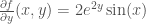
The partial derivative  with respect to , denoted as follows:

is the derivative of  considered as a function of  alone. To find the following:

you must hold  constant (so  is now a function of one variable ), and take the regular derivative of  with respect to . For example, when  is fixed at 1, the preceding function becomes:

This is just a function of one variable , whose derivative is:

In general, thinking of  as fixed, the partial derivative of  with respect to  is calculated as follows:

Similarly, if we hold  fixed instead, the partial derivative of  with respect to  is:

Intuitively, a partial derivative tells you how much the function changes when you perturb one variable a bit. In the preceding example:

So when you start at (0,1), hold  constant, and move  a little,  changes by about 7.4 times the amount that you changed .

As stated above, in machine learning, partial derivatives are mostly used in conjunction with the gradient of a function (when there are multiple weights).

Gradient of a Function (Machine Learning)

The gradient of a function, is the vector of partial derivatives with respect to all of the independent variables:

∇f

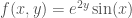
For instance, if:

then:

Note the following:

∇f	Points in the direction of greatest increase of the function.
−∇f	Points in the direction of greatest decrease of the function.

The number of dimensions in the vector is equal to the number of variables in the formula for f; in other words, the vector falls within the domain space of the function. For instance, the graph of the following function:

when viewed in three dimensions with  looks like a valley with a minimum at (2,0,4):

The gradient of  is a two-dimensional vector that tells you in which  direction to move for the maximum increase in height. Thus, the negative of the gradient moves you in the direction of maximum decrease in height. In other words, the negative of the gradient vector points into the valley.

In machine learning, gradients are used in gradient descent. We often have a loss function of many variables that we are trying to minimize, and we try to do this by following the negative of the gradient of the function.

Peak Value (Audio)

The Peak Value is the highest voltage that the waveform will ever reach, like the peak is the highest point on a mountain.

Room Mean Square — RMS (Audio)

The RMS (Root-Mean-Square) value is the effective value of the total waveform. It is really the area under the curve. In audio it is the continuous or music power that the amplifier can deliver. For audio applications, our ears are RMS instruments, not peak reading so using RMS values makes sense, and is normally how amplifiers are rated.

Installing TensorFlow on a MacBook Pro

Introduction

I want to write Machine Learning (ML) applications and so I need to select tools that will help me do this.  I have very little practical experience and so the purpose of this post is to show my discovery process in the hope that it also helps others on the same path.

TensorFlow

I have a strong desire to one day take advantage of Google’s Tensor Processing Unit (TPU).  Clearly Google is aggressively re-positioning itself as a Artificial Intelligence (AI) company; they are hiring a large number of top resources, they are leading certain types of research (such as with DeepMind), they are creating cloud-based services such as Google Cloud ML, they are incorporating ML into all their products, and with TensorFlow they have created an open-source software library for Machine Intelligence.  To me, the attraction of using TensorFlow and the TPU includes:

1. It leverages Google’s AI work and experience.
2. It simplifies the development process by having the same company providing the library, processors etc.
3. I can leverage the significant ML cloud infrastructure being built by Google.
4. Google’s technologies are largely platform neutral and I would like to have that flexibility.
5. Given the presence of Google, open source resources will gravitate to TensorFlow and therefore accelerate its on-going development.

Alternatives to TensorFlow

Major alternatives to this includes Torch and Theano.  Torch is framework written in Lua and is extensively used at Facebook’s AI Research Laboratory (FAIR), Twitter Cortex and NVIDIA.  Facebooks’s Yann LeCun is an important AI pioneer and his research papers, such as the latest on Tracking The World State with Recurrent Entity Networks, are very important in the development of AI.  NVIDIA are key in providing GPUs and supercomputers for AI projects (such as the NVIDIA DGX-1 recently given to OpenAI).  Torch and NVIDIA are a very strong combination and should seriously be considered for ML development.  If following this path, it would be advisable to use Ubuntu as most of the NVIDIA tools, such as DIGITS and their Deep Learning Software, use Ubuntu as the preferred operating environment.

Theano is a Python library and is used by the Montreal Institute for Learning Algorithms (University of Montreal), one of the leading AI research universities.  Theano is one of the oldest complete libraries available; TensorFlow is considered the next generation improvement over Theano.

These libraries have their attractions, with Torch being the most interesting.  So, although I will initially gravitate towards TensorFlow, it will also be important to continuously monitor developments in Torch and NVIDIA and no doubt this will become part of my toolkit.

Installing TensorFlow

My software development environment includes a MacBook Pro (Retina, 15-inch, Mid 2015) running macOS Sierra version 10.12.3 and homebrew.  This version of the MacBook Pro does not have a NVIDIA GPU therefore I cannot install a version of TensorFlow with GPU support.

In the longer term I plan to use Google’s Go Programming Language for software development.  There is a Go binding to TensorFlow but this is currently experimental; the TensorFlow Python API is the most complete therefore I will use that.  The TensorFlow Python API supports Python 2.7 and Python 3.3+ so it is assumed you have already installed Python and pip via homebrew.  The steps to install TensorFlow (without GPU support) are:

$ sudo easy_install pip
$ sudo easy_install --upgrade six
$ pip install tensorflow

Once this is completed then you should be able to test the TensorFlow implementation by running:

$ python
...
>>> import tensorflow as tf
>>> hello = tf.constant('Hello, TensorFlow!')
>>> sess = tf.Session()
>>> print(sess.run(hello))
Hello, TensorFlow!
>>> a = tf.constant(10)
>>> b = tf.constant(32)
>>> print(sess.run(a + b))
42
>>>

If you choose to install from source you will need to:

1. Install Bazel .
2. Install the Python dependencies.

Bazel is an open source tool that allows for the automation of building and testing of software.  Google uses Blaze as its internal build tool and released and open-sourced part of the Blaze tool as Bazel.  To install Bazel and the Python dependencies, run the following:

$ brew install bazel
$ brew upgrade bazel
$ sudo easy_install -U six
$ sudo easy_install -U numpy
$ sudo easy_install wheel
$ sudo easy_install ipython

Next you will need to clone and configure the repository as follows:

$ git clone https://github.com/tensorflow/tensorflow
$ ./configure

When configuring I would activate Google Cloud Platform support and of course there is no GPU on my system.  Once configuration is complete you can build TensorFlow (without GPU support) as follows:

$ bazel build -c opt //tensorflow/tools/pip_package:build_pip_package
$ bazel-bin/tensorflow/tools/pip_package/build_pip_package /tmp/tensorflow_pkg
$ sudo pip install /tmp/tensorflow_pkg/tensorflow-0.xx.x-py2-none-any.whl

You will need to ensure that the name of the .whl file matches the current version.  You can then test the installation as follows:

bazel build -c opt //tensorflow/tools/pip_package:build_pip_package
mkdir _python_build
cd _python_build
ln -s ../bazel-bin/tensorflow/tools/pip_package/build_pip_package.runfiles/org_tensorflow/* .
ln -s ../tensorflow/tools/pip_package/* .
python setup.py develop

You can then test this implementation by running:

$ cd /usr/local/lib/python2.7/site-packages/tensorflow/models/image/mnist
$ python convolutional.py

A full description on how to download and setup TensorFlow for your platform can be found here.

Installing Torch

There are many suggestions for installing Torch but on macOS it is best to follow the standard installation process provided on the Torch site here.

Last Weekend in Ceske Krumlov..cloudy..

České Budějovice – June 2016

plantage.menu – life for 12 months

Ceske Krumlov

České Budějovice – A Room

Vienna, March 2016

České Budějovice in February

Taken on an iPhone 6s Plus.

České Budějovice and Jindřichův Hradec

České Budějovice – Square of Přemysl Otakar II

Jindřichův Hradec – iPhone 6s Plus photos at sunset